Difference Analysis
Now that you have gained an overview of your process, you can start your in-depth analysis on the PAFnow Difference Analysis Page. You can compare key figures of process paths, for example the process performance of different years. This way you can learn more about possible process variants and whether there are differences in the process related to a specific attribute.
Agenda
- The PAFnow Process Explorer on this page, right next to the menu. The process flow is colored based on your attribute selection. You can use every attribute with categorical values as a legend.
- A navigation bar on the right, helps you further control the process flow to receive more specific evaluations
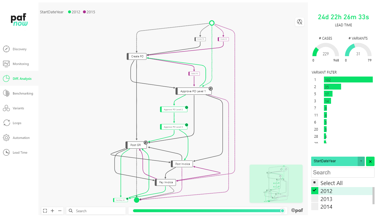
In the example above we compare the two processes depending on their start year. We compare two years: 2012 (green) and 2015 (purple). The grey paths can be found in both years. As you can see, the activity Create SC occurred only in 2015 whereas Approvals of Level 2 happened only in 2012.
Of course, you can compare more than two paths and look at many more attributes in your difference analysis defining the values of your interest with the PAFnow Attribute Filter.
Navigation Bar
Lead Time
The average total lead time is visualized with the PAFnow Duration Card. In the example, the Lead Time of the entire process is displayed:
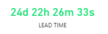
You can also choose more specific lead times, e.g. for particular process steps and can decide how granular the format should be (in days, hours, minutes or seconds). The example above is very detailed and shows the time up to the level of seconds.
In the example, the process in the years 2012 and 2015 took an average of 24 days, 22 hours, 26 minutes and 33 seconds.
Cases & Variants
The gauge visualizations show you the absolute number of currently filtered and displayed cases and variants. If you change the filters, for example by adding one more year to your difference analysis in the Attribute Filter, the number of cases and variants, as well as the average lead time will be newly calculated.
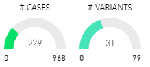
In the example, we can see that in 2012 and 2015, there were 229 cases which caused 31 different variants.
Variant Filter
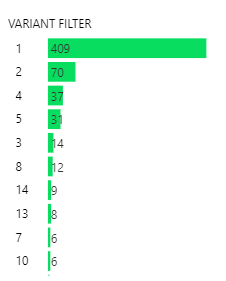
The PAFnow Variant Filter gives you the option to filter for an individual or more variants.
Info
The top variant with the ID 1 is the most frequent variant found in the complete data set (see details in Discovery Page).
However, on the Difference Analysis Page, there is a filter for only the cases of the years 2012 and 2015. This means the frequency of the cases which belong to a particular variant might differ from the frequency distribution of all cases without any active filters. Here you can see that the order of the variant IDs is no longer ascending and sorted by the ID itself but by the ascending number of cases for each variant. For example, VariantId 3 is the third most frequent variant for the complete data but in the selection of only 2012 and 2015 it is only the fifth most frequent variant.
Attribute Filter
Using the PAFnow Attribute Filter, you can filter by selected attributes to see how the process, as well as other evaluations and key figures, will behave for your chosen selection.
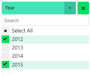
Here, two years are selected. You can easily add one or more years by checking the box(es).
Legend Feature
If you want to compare not only the process for different years but also for other attributes, you can simply add more attributes to the Attribute Filter and change the legend for the Process Explorer.
Info
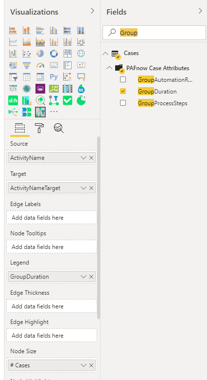
If you want to change the legend, you can simply drag any other case attribute into the legend field of the Fields area in the Visualization pane.
In the same way, you can add an attribute to the PAFnow Attribute Filter.
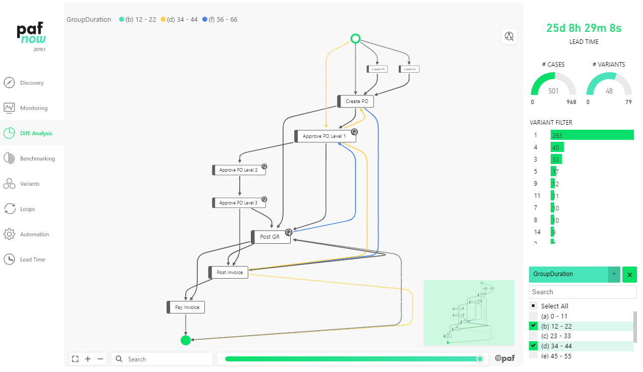
By selecting several values of the chosen attribute (here: Group Duration) you can compare your process accordingly. For example, you can see that the loop from Post GR to Approve PO Level 1 only happens for cases in category (e) which is a lead time between 56 to 66 days.